Concrete is one of the most used building materials in the world. Due to being both cheap and strong it is commonly used in buildings, dams and roads. Concrete is a composite material, composed of a mixture of mainly cement, water and construction aggregate (gravel and sand of varying size). In so called high-performance concrete additional materials are included in the mix to improve the properties of the concrete.

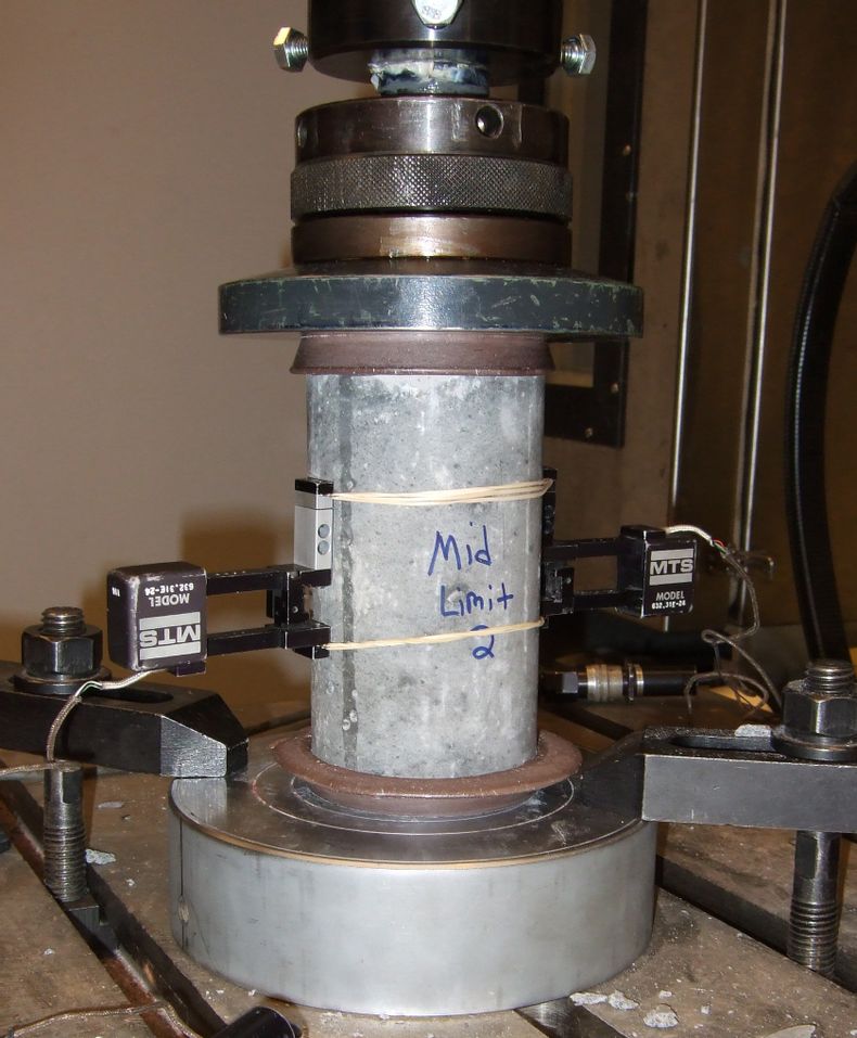
Understanding the properties of concrete is important in order to use it in a safe and efficient way. We will look at a scenario where you have been tasked by a concrete producer to help them optimize their product. In particular, they want to find a mix of high-performance concrete that maximizes the compressive strength of the material. The compressive strength is how much pressure a material can withstand when being pressed together. The image below shows a setup for testing the compression strength of concrete.

Your task in the process of optimizing the concrete mixture is to use machine learning to build a model for the compressive strength. Having a model that can predict the compressive strength of a specific concrete mixture reduces the amount of experiments that have to be made, saving both time and money for the company.

It is well known that the relationship between the amount of each material in the mixture and the compressive strength is highly non-linear. Using a neural network for this task could be a suitable approach, given that you have access to enough data.

A similar concrete study was done in 1998, where I-Cheng Yeh collected a dataset of different concrete mixtures and modelled their compressive strength using neural networks (Yeh, 1998). The collected dataset was kindly made available online and you choose to use it also for your study. Since the original study was done in 1998, more modern approaches to using neural networks are available to you. Making your own model also means that the company can use it freely in their future concrete experiments.

The concrete dataset consists of 1030 different concrete mixtures with associated compressive strengths. The features of each data point are the amount (kg/m$^3$) of each material in the mixture. The materials in the mixture are:

• Cement
• Blast furnace slag
• Fly ash
• Water
• Superplasticizer
• Coarse aggregate
• Fine aggregate

Additionally, the compressive strength depends of the age of the concrete (how long ago it was mixed). Each data point has an additional age feature, describing how many days that had passed from the cement was mixed to the compressive strength was measured. Using this as an input feature means that your model will not just learn the compressive strength of a specific mixture, but also how this depends on the age of the material. In total this adds up to 8 features per concrete mixture. The target variable is the compressive strength of the concrete, which is a single scalar value measured in Megapascal (MPa).

The dataset is already pre-processed by normalizing all features and split into:

• Training set of 618 samples (60%)
• Validation set of 206 samples (20%)
• Test set of 206 samples (20%)

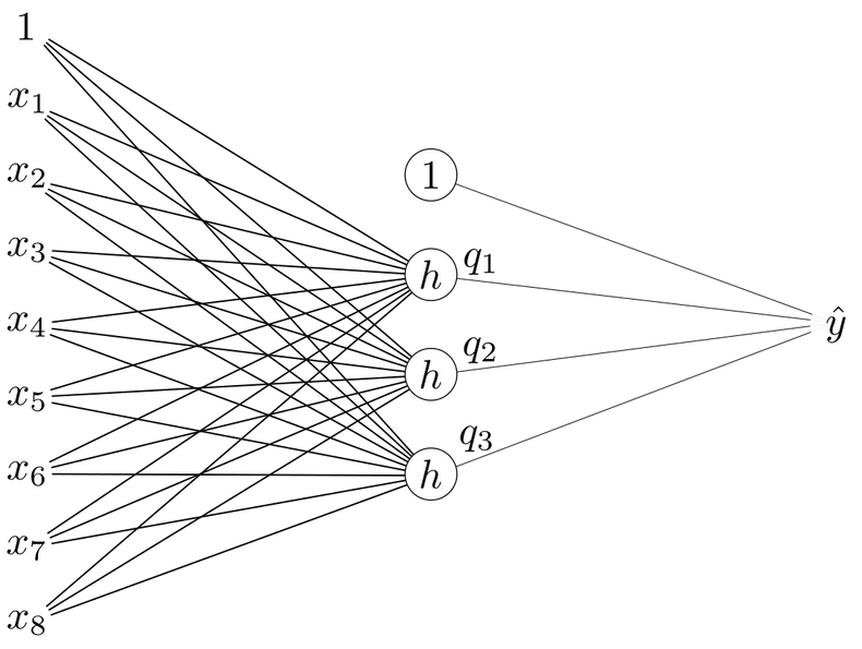
Your first neural network model will have a single hidden layer containing 3 units. The hidden units use ReLU activations:

and the single output unit does not apply any activation function. A figure describing the architecture is given below.

How many parameters does this neural network have in total (weights + offsets/biases)? If we stack all network parameters in a vector $\mathbf{\theta}$ this would be the dimensionality of this vector.

Before we start working with this model in code let’s brush up on how the neural network model works.

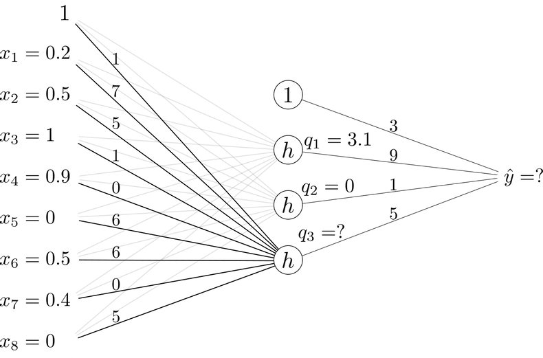
Below, a neural network with the structure introduced in the previous question is illustrated. The weights and offsets of the network are given, as well as the values of the two hidden units obtained for the given input.

Compute the value of the last hidden unit $q_3$ (after the ReLU activation has been applied). Give your answers with one decimal place.

Using the same neural network and input as in the previous calculation, compute the network output $\hat{y}$. Give your answer with one decimal place.

Let us now build this neural network in code. We will once again make use of scikit-learn, that contains a few classes of neural network models. We are here solving a regression problem and will again use the squared error cost function. A neural network model trained using this cost function is implemented in the MLPRegressor class of scikit-learn. MLP here stands for Multilayer Perceptron, which is just another name for a standard neural network with at least one hidden layer. Since there are many design choices involved with building and training a neural network model, the MLPRegressor class has a large number of parameters. Although we will only make use of a few of them here, you can find the full list in the documentation.

• The adam optimizer (denoted solver in scikit-learn) should be used for training.
• The model should be trained for 3000 epochs (iterations).
• The size of each mini-batch should be set to 128.
• The initial learning rate should be set to 0.005. Recall that the optimizer will adapt the learning rate during the training process.

Note that the MLPRegressor class uses $L^2$-regularization with a coefficient 0.0001 by default. We will leave it at that value. After creating the model, train it using the training split of the dataset. Also use the given function to plot the training loss curve. This describes how the loss (calculated on the training set) changes over the 3000 training epochs.

Run the code below to evaluate the model on the validation set.

This first architecture with a single hidden layer of three units is quite simple to understand and we could even do some calculations using it by hand (given the weights). However, knowing that there are complex non-linear relationships in the data we could likely benefit from using an even more flexible model. To see if this can improve our results, we will now scale up our neural network architecture to more layers and units.

Create a new neural network model, this time with 3 hidden layers of 512 units each. Train and evaluate the model in the same way as before. Leave all other hyperparameters at the same values.

As we can see, using a more flexible model here improves our predictions on the validation set. Happy with this model, we can finally evaluate it on the test split of the dataset.

The error on the test set is your final estimate for the expected future error of the model. You report this to the customer and they seem happy with your results. Your model will be highly useful in their work on optimizing the concrete mixture.

As we saw in Question D, scaling up the neural network model substantially improved our results. As we have seen many times throughout the course, a key problem in using machine learning is to match the flexibility of the model to the dataset at hand.

We reduced the error when scaling up the model in question D, but why stop there? We could of course build an even bigger neural network, with more hidden layers and more units in each layer. What is the main reason that we should not expect better results if we just keep scaling up our model indefinitely?

In this example we have looked at using neural networks for a somewhat low-dimensional ($\mathbf{x}$ had 8 dimensions) regression problem. This is one setting where neural networks can be very useful, in particular if we have complex non-linear relationships between $\mathbf{x}$ and $y$. In the low-dimensional setting we could have easily considered other types of models as well, for example k-Nearest Neighbor or polynomial regression. While we don’t know exactly how these would perform on this dataset, they are still suitable choices for this general type of problem. Another setting where neural networks are especially useful is when $\mathbf{x}$ is very high-dimensional. In these cases many other machine learning models struggle, either because they are not flexible enough or because the computational cost makes them impossible to use in practice. In the next example we will look at one such dataset. We will consider images of $64 \times 64$ pixels, making $\mathbf{x}$ 4096-dimensional. We will also see how convolutional neural networks allow us to build models that work with such high-dimensional data.